from matplotlib import plt
Caspan = np.linspace(0,2,100)
plt.plot(Caspan, steady(Caspan),linewidth=2)
plt.legend(('$f(x)=F_{a0}-vC_a+\\frac{1.75VC_a}{(1+10C_a)^2}$',),0,fontsize=18, shadow=True)
plt.plot(Caspan,np.linspace(0,0,100),'k-',linewidth=1)
plt.plot(Cas[0],0,'ko',Cas[1],0,'ko',Cas[2],0,'ko',markersize=7)
plt.plot(np.linspace(Cas1,Cas1,100),np.linspace(-0.15,0,100),'k--',linewidth=2)
plt.plot(np.linspace(Cas2,Cas2,100),np.linspace(-0.15,0,100),'k--',linewidth=2)
plt.plot(np.linspace(Cas3,Cas3,100),np.linspace(-0.15,0,100),'k--',linewidth=2)
plt.text(Cas[0]-0.02, 0.03, str(round(Cas[0],3)) + ' $mol/L$ ',fontsize=14)
plt.text(Cas[1]+0.05, -0.02, str(round(Cas[1],3)) + ' $mol/L$ ',fontsize=14)
plt.text(Cas[2], 0.01, str(round(Cas[2],3)) + ' $mol/L$ ',fontsize=14)
plt.xlabel('$C_a (mol/L)$',fontsize=16)
plt.ylabel('$f(x)$',fontsize=16)
plt.title('Plot of the Target Function', fontsize = 20)
plt.savefig('images/cstr-mult-steady-state-1.png')

fig = plt.figure()
ax1 = fig.add_subplot(111)
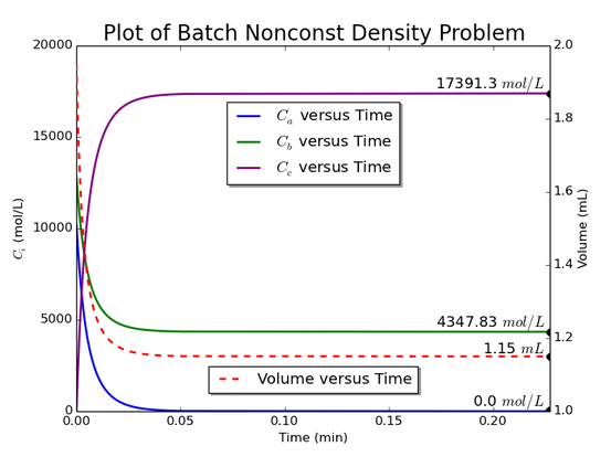
ax1.plot(tspan, Caspan,'b',label= "$C_a$ versus Time",linewidth = 2)
ax1.plot(tspan, Cbspan,'g',label= "$C_b$ versus Time",linewidth = 2)
ax1.plot(tspan, Ccspan,'purple',label= "$C_c$ versus Time",linewidth = 2)
ax1.legend(loc=8, bbox_to_anchor = (0.5, 0.6), shadow=True)
ax1.set_xlim(0, tspan[-1,0])
ax1.set_ylim(0, 20000)
ax1.set_xlabel('Time (min)')
ax1.set_ylabel('$C_i $ (mol/L)')
ax2 = ax1.twinx()
ax2.plot(tspan, V*1000, 'r--',label = "Volume versus Time",linewidth = 2)
ax2.legend(loc=8, bbox_to_anchor = (0.5, 0.03), shadow=True) # Make volume in the unit of mL.
ax2.set_ylabel('Volume (mL)')
ax2.set_xlim(0, tspan[-1,0])
ax2.set_ylim(1, 2)
ax1.plot(tspan[-1], Caspan[-1], 'ko',markersize=9)
ax1.text(tspan[-1], Caspan[-1], str(round(Caspan[-1],2)) + ' $mol/L$ ',fontsize=14, horizontalalignment='right', verticalalignment='bottom')
ax1.plot(tspan[-1], Cbspan[-1], 'ko',markersize=7)
ax1.text(tspan[-1], Cbspan[-1], str(round(Cbspan[-1],2)) + ' $mol/L$ ',fontsize=14, horizontalalignment='right', verticalalignment='bottom')
ax1.plot(tspan[-1], Ccspan[-1], 'ko',markersize=7)
ax1.text(tspan[-1], Ccspan[-1], str(round(Ccspan[-1],2)) + ' $mol/L$ ',fontsize=14, horizontalalignment='right', verticalalignment='bottom')
ax2.plot(tspan[-1], V[-1]*1000, 'ko',markersize=7)
ax2.text(tspan[-1], V[-1]*1000, str(round(V[-1]*1000,2)) + ' $mL$ ',fontsize=14, horizontalalignment='right', verticalalignment='bottom')
plt.title('Plot of Batch Nonconst Density Problem', fontsize = 20)
fig.savefig('images/batch-nonconst-density.png')
plt.show()
 RSS Feed
